How to Read a Coefficent Plot R
Interpreting ACF or Machine-correlation plot
Fourth dimension serial is linearly related to a lagged version of itself.
What is ACF plot ?
A fourth dimension series is a sequence of measurements of the same variable(southward) fabricated over time. Usually, the measurements are made at evenly spaced times — for example, monthly or yearly. The coefficient of correlation between two values in a time serial is called the autocorrelation office (ACF). In other words,
>Autocorrelation represents the degree of similarity between a given fourth dimension series and a lagged version of itself over successive time intervals.
>Autocorrelation measures the relationship betwixt a variable'due south current value and its past values.
>An autocorrelation of +1 represents a perfect positive correlation, while an autocorrelation of negative 1 represents a perfect negative correlation.
Why useful ?
- Help us uncover hidden patterns in our data and help united states select the correct forecasting methods.
- Assistance identify seasonality in our time series data.
- Analyzing the autocorrelation function (ACF) and fractional autocorrelation function (PACF) in conjunction is necessary for selecting the appropriate ARIMA model for any fourth dimension series prediction.
Whatsoever supposition made by ACF ?
Weak stationary — meaning no systematic alter in the mean, variance, and no systematic fluctuation.
So when performing ACF information technology is advisable to remove whatever trend nowadays in the information and to make certain the data is stationary.
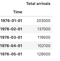
Try out with a real dataset?
          data = pd.read_csv('data.csv',
            engine='python',parse_dates=[0],
            index_col =            'Time',
            date_parser = parser)st_date = pd.to_datetime("2008-01-01")
data = data[st_date:]
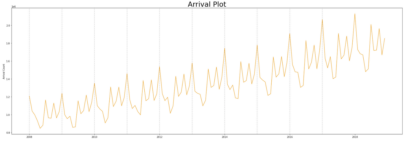
The plot of the data looks similar beneath:
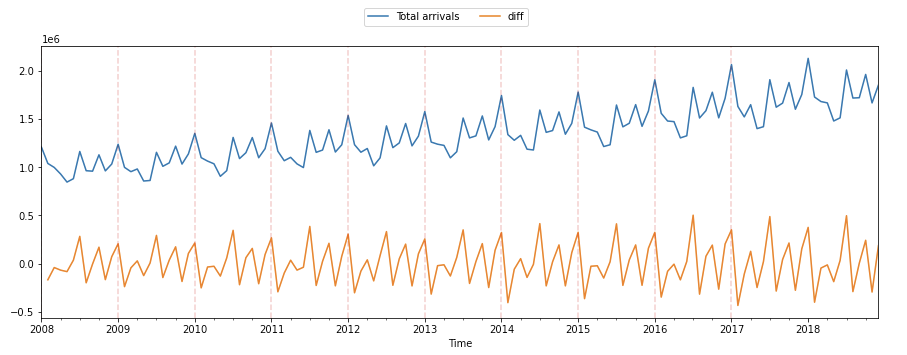
At present, before performing the ACF let's remove the tendency and encounter how information technology looks like:
                      #acf -> remove trend
            data["unequal"] = data.diff()ax = data.plot()
ax.legend(ncol=5,
              loc='upper center',
              bbox_to_anchor=(0.5, 1.0),
              bbox_transform=plt.gcf().transFigure)
              for              year              in              range(2008, 2018):
              ax.axvline(pd.to_datetime(str(twelvemonth)+"-01-01"), colour ="ruddy", linestyle =              "--", blastoff = 0.two)
Now allow'south utilise the ACF:
                      from            statsmodels.graphics.tsaplots            import            plot_acf
data["diff"].iloc[0] = 0
plot_acf(data["unequal"])
plt.bear witness() 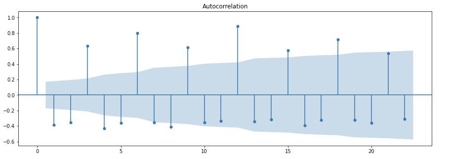
Tin you lot come across the seasonality present?
Notice how the coefficient is high at lag three, vi,9,12. In terms of the month if I have to say then, high positive correlations for March, June, September, December, whereas Jan, February and Apr take negative correlations but that likewise vanishes with lag. Nosotros will focus on the points that lie beyond the blue region as they signify strong statistical significance.
Of import note: make sure your data doesn't accept NA values, otherwise the ACF volition fail.
Tin we wait at the tendency and seasonality separately to dive deep into the data?
Yeah, let's decompose the data. I am going to use a stats model API for this purpose merely ane tin can employ NumPy and Pandas besides to decompose the three parts of a time series -tendency, seasonality, balance.
                      from            statsmodels.tsa.seasonal            import            seasonal_decomposeres = seasonal_decompose(data, model =              "condiment",period = 30)            fig, (ax1,ax2,ax3) = plt.subplots(3,1, figsize=(15,8))
res.trend.plot(ax=ax1,ylabel =              "trend")
res.resid.plot(ax=ax2,ylabel =              "seasoanlity")
res.seasonal.plot(ax=ax3,ylabel =              "residual")
plt.bear witness()
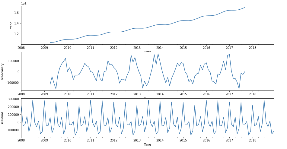
Notice how I chose additive instead of multiplicative since there is no exponential increase in the amplitudes over time.
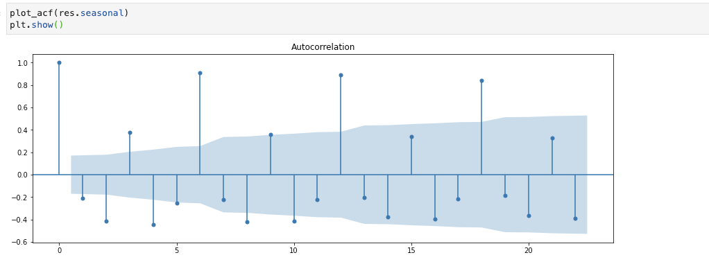
Now if I run the aforementioned ACF plot on the res.seasonal component generated by the API we will go the same coefficients every bit before.
Source: https://medium.com/analytics-vidhya/interpreting-acf-or-auto-correlation-plot-d12e9051cd14
0 Response to "How to Read a Coefficent Plot R"
Enregistrer un commentaire